This paper presents a sensor fusion algorithm for estimating the flight parameters of an Unmanned Micro Air Vehicle is presented. The sensor fusion algorithm is illustrated through simulation using a nonlinear six-degree-of-freedom model of the aircraft and simple sensor models.
Keywords: sensor fusion, GPS errors, INS errors

1. INTRODUCTION

Sensor fusion is a method for conveniently integrating data provided by various sensors, in order to obtain the best estimate for a dynamic system's states. Sensor fusion algorithms are particularly useful in low-cost UAV applications, where acceptable performance and reliability is desired, given a limited set of inexpensive sensors. The sensor fusion system can provide: filtered high-rate navigation and control data for increased performance, estimation of the flight parameters which are not measured directly (i.e. attitude angles, angle-of-attack, sideslip), detection of significant changes in aircraft dynamics (i.e. icing, airframe damage), and the ability to replace failed sensor outputs with estimates (graceful degradation).

The aim of this research work is to study the applicability of various sensor fusion algorithms for different airplane configurations. The performance of the sensor fusion algorithms will be tested in simulation using models of the aircrafts and sensors.

2. MODELS

For simulation purposes, a nonlinear 6-degree of freedom model was developed, for use in the Matlab/Simulink environment - Fig.1. The model includes Simulink blocks for the equations of motion, aerodynamics, propulsion, inertia, standard atmosphere, background wind, turbulence, and a WGS-84 Earth model [1]. The aerodynamics is based on look-up tables of wind tunnel test results. The aerodynamic coefficients of the models were obtained from the Slope Soaring Simulator [1]. The Slope Soaring Simulator is an open-source flight

The propulsion model is based on propeller wind tunnel tests and engine experimental data.

The simulator model takes the following inputs:

• Actuators: control surfaces - flap, elevator, aileron, rudder deflections, as well as throttle setting;
• Atmospheric conditions: background wind vector, turbulence intensity, sea-level pressure and temperature.

The model outputs the following parameters:

• Aircraft states: body-axes velocities, angular rates, attitude angles, position and engine speed;
• Aircraft sensors: position and groundspeed, accelerations, angular rates, and air data (static pressure, dynamic pressure and outside air temperature);

Figure 1: The Simulink Model

• Aerodynamic coefficients;
• Propeller coefficients;
• Engine parameters;
• Wind-axes velocity components: airspeed, sideslip angle and angle-of-attack;

Linear position - East, North, Up components, relative to the starting point.

The basic sensor set which will be used includes a low cost GPS receiver providing position and groundspeed information at a rate of 4 Hz, 3 accelerometers and 3 rate gyros providing a complete 6-degree of freedom inertial solution, and an air data system which outputs static and dynamic pressure as well as the outside-air temperature.

Simple dynamic models for the sensors were created for simulation purposes. The sensor models were implemented as Simulink blocks and have the following features: white noise, offset drift, scale factor variation, and saturation limits.

The simulation set-up is shown in Fig. 2. The aircraft model can be controlled by fixed actuator commands, manual control using a joystick, or automatic control from an autopilot block. The ideal sensor signals that the aircraft model outputs are corrupted by the sensor model blocks, and then fed to the sensor fusion block, which estimates the aircraft states. The estimated states are then plotted against the actual aircraft states returned by the simulator. This simple comparative plot has the advantage that not only can we see the magnitude of the estimation error relative to the magnitude of the signal, but we can correlate the variation in estimation performance with various aircraft maneuvers during the flight.

Using these simulations set-up we will analyze the performance of the sensor fusion algorithm which is presented next.

Figure 2: The simulation set-up

3. Considerations about the GPS / INS integration

            The INS algorithm integrates the accelerations and angular rates provided by an Inertial Measurement Unit (IMU) to compute the position, velocity, and attitude (PVA) of the vehicle. The algorithm takes into account the Earth rotation rate and geodic shape, and it also includes a gravity model.

An INS algorithm by itself is seldom useful since the inertial sensor biases and the fixed-step integration errors will cause the PVA solution to diverge quickly. The navigation system must account for these error sources to be able to correct the PVA estimate.

A low-cost GPS (Global Positioning System) receiver can output the aircraft position and groundspeed. The measurement will be corrupted by time-correlated noise and provided at a low rate, typically 1 Hz - not fast enough for some flight control applications. Also, the GPS signal is susceptible to jamming. However, the position and velocity measurements do not drift over long periods of time.

            A low-cost IMU (Inertial Measurement Unit) can output the aircraft accelerations and angular rate which can be integrated by an INS to obtain the aircraft position, velocity, and attitude. The IMU measurements are corrupted by noise, scale factor and bias variations with temperature (nonlinear, difficult to characterize). By integrating the IMU measurements with the INS algorithm, the errors will accumulate, leading to significant drift in the position and velocity outputs. One advantage of the IMU is that it can be sampled at high-rates, therefore it is capable to capture the fast dynamics of the aircraft. But the main advantages over GPS is that the INS is autonomous (does not rely on any external aids), it is immune to jamming and inherently stealthy (does not emit nor receives any detectable radiation).

The disadvantages include the following:

1. Mean-squared navigation errors increase with time.
2. Cost, including:

a)      Acquisition cost, which can be an order of magnitude (or more) higher than GPS receivers.
b)      Maintenance cost.

3. Power requirements, which have been shrinking along with size and weight but are still higher than those GPS receivers.
4. Heat dissipation, which is proportional to and shrinking with power requirements.

The advantages and disadvantages of the GPS and INS sensor systems makes them complementary, and the best estimates of the aircraft position, velocity and attitude can be obtained by combining both GPS and INS measurements using the GPS/INS integration method presented below.

4. THE SIMULATION SETUP AND RESULTS

To setup the simulation we had to implement two models:

1. The GPS model
2. The IMU model

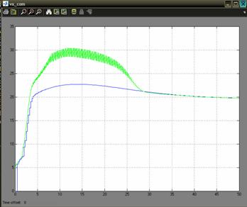
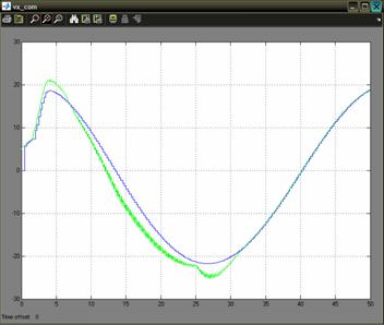
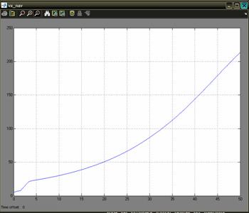
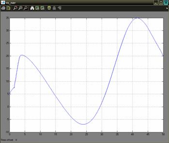
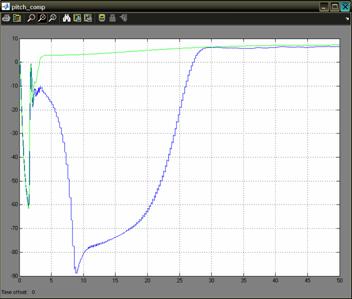
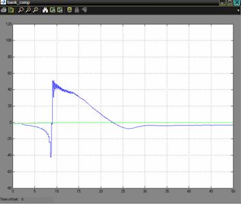
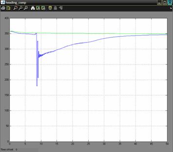
            The data obtained is processed by a navigation filter.

The outputs of the GPS model are the position and the velocity at a rate of 4 Hz. The IMU model defines the biases and the noise for the accelerometers and gyros. The navigation filter simulation sample time is set to 0.05 s.

The estimated parameters of the UAV are computed by the navigation filter, using the outputs of the GPS and IMU model. Also, the GPS outputs are ploted to compare the simulated results with the one obtained from the navigation filter. The model takes as input commands the airspeed command which was setup to the constant value of 20 m/s and the bank angle command which is set to the value of 0⁰. The wind velocity is set to zero for all the three axes, but it can be modified. The simulation time is set to 50 seconds. The results are presented in Figure 3.The blue line represents the simulated value for the groundspeed on x-axis, and the green line is the one obtained from the navigation filter. Similar results are obtained for the y-axis and z-axis.

Figure 3: Simulation results for 0⁰ bank angle

A second simulation was made, in which the command for the bank angle is set to 15⁰. The results are shown in Figure 4.

Figure 4: Simulation results for 15⁰ bank angle

Another interesting simulation is the one regarding the estimation of the speed using only the information provided by the IMU unit model without the correction provided by the GPS model. The outputs of the sensors of the unit are corrupted with noise, and also other characteristics like the offset drift, scale factor variation, and saturation limits are modeled to simulate a real IMU. It is expected a divergent behavior of the estimate of the speed.

Like in the precedent case, two cases will be studied: a one in which the bank angle will be set to 0⁰ and the second one for a bank angle of 15⁰. Of course, other cases can also be studied for other values of the bank angle.

The results for the first case are presented in Figure 5.

Figure 5: GPS off, bank angle 0⁰

The results for the second case are presented in Figure 6.

Figure 6: GPS off, bank angle 15

In the first case the divergence of the estimate is increasing in time with a higher rate than in the second case.  This is caused by the different modes of the accumulation in time of the error.

Another important problem regards the determination of the attitude. For the 0⁰ angle of bank command were made simulations which show the three angles of the attitude, the bank angle, the pitch angle, and the angle of heading. The simulations are ploted in Figure 7 a, b, c. The results are computed by the navigation filter (blue line) and ploted against the simulated ones (green line).

a)      the results for the pitch angle

b)      the results for the bank angle

c) the results for the heading angle

Figure 7

In all the there figures we can see that the filter takes a time to stabilize itself. This period is about 30 seconds. This is due, to the covariance of the outputs of the sensors. After this period the results estimated by the navigation filter are following closely the real ones.

5. Conclusions

            In all the graphics presented above it can be seen that the simulated filter has a period of transition in which the covariance needs to stabilize. For applications where high maneuverability is required the filter is not suitable. If a mission where waypoints fly is needed and where the demands for maneuverability are not a stringent problem the filter can be used to estimate the position and the attitude. Although future work must be done in order to optimize the results for the period of transition.

Acknowledgments

I would like to acknowledge mister engineer Marius NICULESCU from Unmanned Dynamics for his priceless support which was decisive in conceiving this paper.

References

[1] AEROSIM BLOCKSET Version 1.2 User's Guide Unmanned Dynamics, LLC.

[2] Mohinder S. Grewal, Lawrence R. Weill, Angus P. Andrews, Global Positioning Systems, Inertial Navigation and Integration, John Willy & Sons Inc., 2001.

[4] Boscoianu, M. "Some aspects about the new opportunities offered by a small size HALE UAV", Budapest, International Conference Miklos Zrny Military University, 18-19 oct  2005.

[5] Coman A., Safta D., Boscoianu M. "A Method for Optimising the Stability of Flight Velocity of Modern Aerospace Propulsion Systems" 57th IAC Congress, Valencia, Spain, October 02-06 2006.